
In this tutorial, we will sketch various linkages, and use SolveSpace's geometric constraint solver to simulate their motion. A linkage will consist of at least two parts, constrained to move with respect to each other in some particular way. For example, a two-dimensional linkage may consist of long rigid bars, connected with pin joints at their endpoints. Two bars result in simple circular motion, and three in a rigid truss; so interesting linkages of this form will generally consist of at least four bars.
These linkages are difficult to analyze without a computer. Various general closed form results do exist, but nothing particularly useful. It's easier to let the geometric constraint solver find the solution. By modeling the linkage in this manner, we also can constrain 3d parts against the skeleton of the linkage, and animate the motion of the actual space-filling parts, for example to check for interferences as the linkage is worked.
Here, we will model one of Theo Jansen's linkages for simulated walking motion. It appears as below:
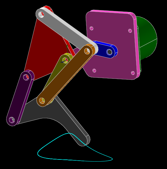
The pink plate is held stationary. The mechanism is driven at the blue link, by the green motor (barely visible behind the pink plate). As the blue link is rotated, the bottom of the grey leg traces the curve in cyan.
To model the linkage, we start with an empty sketch. In that sketch, we will draw and constrain a skeleton of the linkage. A link corresponds to a line segment constrained to a specified length, and a pin joint corresponds to a point-coincident constraint in 2d. (SolveSpace can also sketch in 3d, where that point-coincident constraint would correspond to a ball joint, not a pin joint; but this is a planar linkage, so it's easier to draw in a 2d workplane.) By dragging a link with the mouse, we will be able to work the linkage, analogously to if we applied a displacement at that point in real life, and use various tools to record the resulting motion.
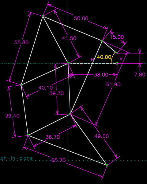
A dimensioned drawing of that skeleton appears as below:
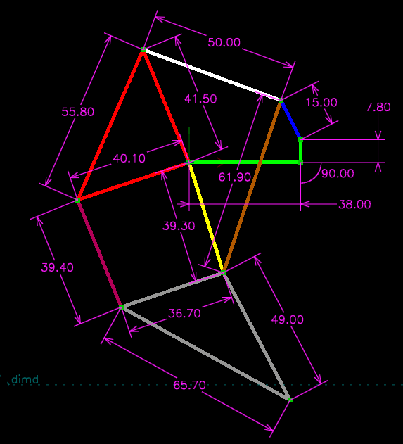
It's an eight-bar linkage (since it consists of eight independently-moving parts); but since the joints on some of those parts don't all lie in a straight line, the sketch consists of more than eight lines, in some cases with a truss structure to provide the extra joint. In the picture, I've marked links that will end up moving as a rigid body in the same color.
To sketch the linkage, we just sketch and dimension those lines as usual. It's helpful to sketch the lines as close as possible to the desired final geometry; it may be possible to assemble the links in a configuration that's different from the desired linkage, and this helps the solver find the intended solution.
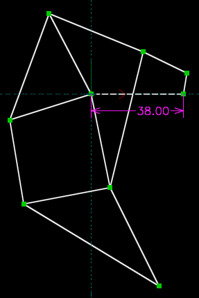
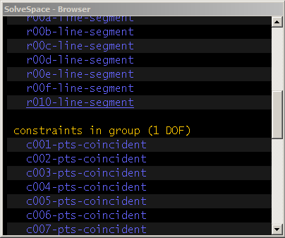
First, we sketch the lines, using Sketch → Line Segment (or keyboard shortcut S, or the corresponding toolbar icon). We can insert some of the point-coincident constraints that join the lines at the endpoints automatically, by clicking an existing endpoint while creating our new line; we also could create them explicitly if desired, by selecting the two endpoints and choosing Constrain → On Point / Curve / Plane. It's helpful to constrain the length of one of the lines before drawing the rest of them, to help get the sketch on the approximately correct scale, and minimize how much it will change when it gets dimensioned.
Then, we insert line length constraints for each link, by hovering the mouse over a link (so that it turns yellow), clicking (so that it turns red), and then choosing Constrain → Distance / Diameter. We double-click each dimension on the sketch, and type in the desired length.
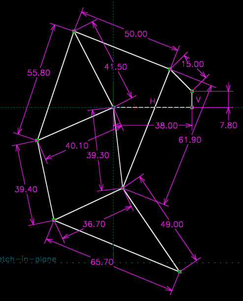
We also constrain the fixed links (drawn earlier in green), by constraining the left end of the horizontal link to lie at the origin (Constrain → On Point / Curve / Plane), and constraining the orientations of the two links (Constrain → Horizontal or Vertical). This fully constrains the linkage; we should therefore have only one degree of freedom, corresponding to the rotation of our driving link. We can confirm this by clicking the home link at the top left of the text browser window, and then clicking the name of the group in which we're sketching, the default "g002-sketch-in-plane".
We can now work the linkage, by dragging a link with the mouse. The solver should generally follow the motion of the mouse. In some cases, the solver may fail and indicate an error, by turning the background of the sketch from black to dark red. This may arise from numerical problems in the solver, in which case we may be able to operate the linkage correctly by dragging slower. It may also arise from a real problem with the linkage; the solver will fail at the same points where a real linkage would bind. In that case, the linkage must be redesigned, or driven from a different link. In any case, the error may be cleared by choosing Edit → Undo.
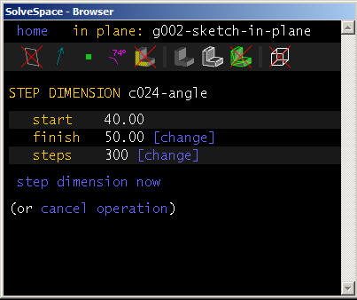
We also can work the linkage with a dimension. For example, we can add a constraint on the angle of the driven link with respect to the long horizontal link, which corresponds to the rotation of the motor or other actuator driving the linkage.
The sketch is now fully constrained, with 0 DOF. To trace the operation of the linkage systematically, we can step that dimension. To do so, we click the dimension (so that it turns red), and then choose Analyze → Step Dimension. The starting angle is determined by that dimension's current value, and we can specify the final angle arbitrarily, by clicking "change" in the text browser window and typing it in, and then hitting Enter. We can likewise specify the number of steps; if we step from 40 degrees to 50 degrees in 20 steps, for example, the solver will move the dimension to 40.5 degrees, then 41, 41.5, 42, ... until it reaches the final value of 50. If we want to watch the linkage move, then we should probably increase that step count, because the solver will otherwise work too quickly for us to see it animate.
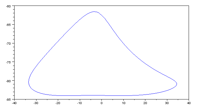
We also can record the position of a point on the linkage as the linkage moves. To do so, we click a point (so that it turns red), and then choose Analyze → Trace Point. Any motion of that point will now be recorded with a cyan curve.
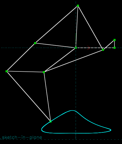
To stop tracing, we choose Analyze → Stop Tracing. A file dialog will appear; we can dismiss that by pressing Escape or choosing cancel, or we can specify a .csv file, into which the points on that trace will be exported, in the model's global (x, y, z) coordinate system. The spacing of those points will be determined by the sequence of positions at which the linkage was solved. If the linkage was worked "by hand", by dragging a link with the mouse, then that spacing will be arbitrary; the geometric curve traced is meaningful, but the speed along that curve is not. Here, for example, the linkage was worked with the mouse, and we then plotted the output point's x as a function of y (in Scilab; but many programs could do this, for example most spreadsheets).
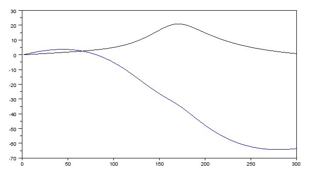
If the linkage was worked with Step Dimension, then that speed is known, and this file may be used to plot output position as a function of link angle. Here, for example, the linkage was worked over a half rotation with Step Dimension, and we plot the change in x (the blue trace) and y (the black trace) as a function of time or, equivalently, angle.
Once the skeleton of the linkage exists, solid models may be constrained against it. This is how the picture at the beginning of this tutorial was generated. If those constraints are chosen appropriately, then the solid models will follow the skeleton of the linkage as the linkage is worked. For a planar linkage, for example, a good choice of constraints is:
- linked part's z-axis normal parallel to our reference z-axis normal, to hold the linked part in a plane parallel to our linkage plane;
- a point from linked part lies in specified workplane (or on specified plane face from solid model), to hold the linked part at the desired translation normal to the plane;
- point-on-point, in 2d (choose a workplane parallel to the linkage plane, and choose Sketch → In Workplane; then select the two points, and choose Constrain → On Point), at one of the pin joints; and
- a line in the solid model parallel to the line in the skeleton of the linkage, also in 2d.
Other combinations of constraints may work, but must be chosen carefully to avoid ambiguity as the linkage moves. To operate the linkage, it's necessary to drag the entities in that original skeleton; this may become difficult as the model becomes crowded with entities from the solid models, since those are easy to instead select by accident. To avoid this, we can hide the entities from those solid models (while leaving the solid model itself visible), by clicking the home link at the top left of the text browser window, and un-checking the "shown" box for those groups.
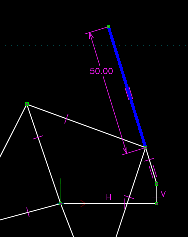
We can also draw a "handle" on the linkage, to extend the driven link and make it easier to grab with the mouse. Here, for example, we do that with an additional line, sharing an endpoint with the driven link and constrained parallel to it. The handle is assigned to a custom line style, so that we can mark it in blue, and hide it in any exported file.
The linkage drawn above used only pin joints. Other kinds of joints may be modeled, using different constraints. For example, a pin that slides in a slot may be modeled as a point-on-line constraint. That constraint is used here, to model a Whitworth quick-return mechanism:
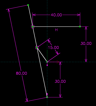
This mechanism contains rotating links: one 15 mm long, about the origin, and one 80 mm long, about a point 30 mm below the origin. As usual, the pin joint for the rotating link in 2d constrains two of the link's three degrees of freedom, leaving it with only rotation about the pinned joint.
It also contains two pins in slots, corresponding to the two point-on-line constraints, drawn here as square magenta boxes. These joints constrain only one degree of freedom, leaving the link free both to rotate about the constrained point, and to translate along the line. Finally, the 40 mm link is constrained horizontal, and 35 mm above the x axis. This corresponds to a linear guide, which constrains two degrees of freedom, leaving the link with only translation in the constrained direction.
As before, we can constrain solid models against the skeleton, and they will follow the motion of the mechanism.
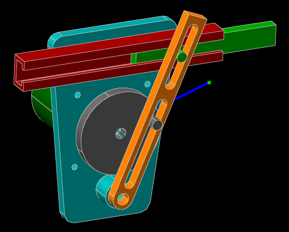
Here, we've once again provided a handle to aid in working the linkage, drawn in blue. The same tools may be used to analyze this linkage as before; everything moves in lines or arcs, so the geometric trace isn't particularly interesting, but the speed of the quick return mechanism, for example, can be measured and graphed, using Analyze → Trace Point on the output point and then Analyze → Step Dimension to work the linkage, and finally Analyze → Stop Tracing to save the results.
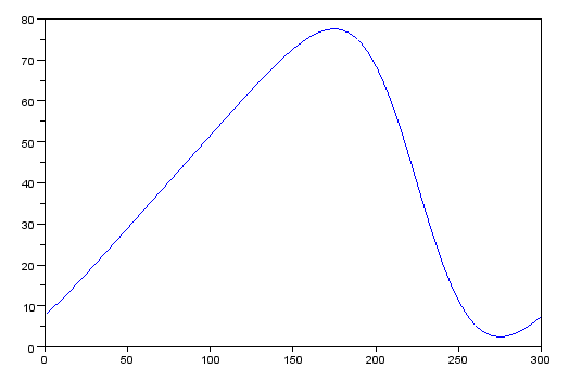
The "quick return" feature is visible here, as the output position increases slowly and then decreases quickly.
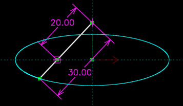
Other mechanisms with linear slides may have more interesting geometric behavior. For example, we can model an elliptical trammel by constraining two points on a line to lie on the x and y axes. Any other point on that line will trace out an axis-aligned ellipse:
The SolveSpace models used in this tutorial are available for download below. Extract all files to the same directory before attempting to open them; some files are assemblies, and will fail to generate if the referenced component files aren't present.