The user interface consists of two windows: a larger window that contains mostly graphics, and a smaller window that contains mostly text. The graphics window is used to draw the geometry, and to view the 3d model. The text window provides information about the model, and may also be used to modify settings and numerical parameters.

Graphics Window and Model View

To pan the view, right-drag with the mouse.

To rotate the view, center-drag with the mouse. This turns the part over, so that the surfaces that used to be hidden (because they were facing backwards, away from the viewer) become visible.

To rotate the view within the plane of the monitor, Ctrl+center-drag with the mouse.

It is also possible to pan by Shift+center-dragging, or to rotate by Shift+right-dragging. If a 3Dconnexion six degree of freedom controller (e.g., a SpaceNavigator) is connected, then this may also be used to transform the view of the model.

To zoom in or out, rotate the scroll wheel. It is also possible to zoom by using the View menu, or the associated keyboard shortcuts (+ and -). Some features, including the planes, are always drawn the same size on-screen, and are therefore not affected by zooming.

Most commands are available in three different ways: from a menu, from a keyboard shortcut, or from the toolbar. The toolbar is displayed at the top left of the graphics window. To learn what an icon means, hover the mouse over it. To show or hide the toolbar, choose View → Show Toolbar.

To zoom to the extent of the part, choose View → Zoom To Fit. This adjusts the zoom level so that the part fits exactly on the screen, and then pans to center the part. The rotation of the part is not affected.

If a workplane is active, then choose View → Align View to Workplane (or press W) to align the view to the workplane. After doing this, the plane of the screen is coincident with the workplane, and the center of the workplane is at the center of the screen. The zoom level is not affected.

In an orthogonal view, one of the coordinate (x, y, or z) axes is horizontal, and another is vertical. To orient the view to the nearest orthogonal view, choose View → Nearest Ortho View. In an isometric view, all three coordinate axes are projected to the same length, and one of the coordinate axes is vertical. To orient the view to the nearest isometric view, choose View → Nearest Iso View.

To pan the view so that a given point is at the exact center of the screen, select that point and then choose View → Center View at Point.

The x, y, and z coordinate axes are always drawn at the bottom left of the graphics window, in red, green, and blue. These axes are live: they can be highlighted and selected with the mouse, in the same way as any other normals. (This means that the coordinate axes are always conveniently available on-screen, which is useful e.g. when constraining a line parallel to the x-axis.)

Dimension Entry and Units

Dimensions may be displayed in either millimeters or inches. Millimeter dimensions are always displayed with two digits after the decimal point (45.23), and inch dimensions are always displayed with three (1.781).

Choose View → Dimensions in Inches/Millimeters to change the current display units. This does not change the model; if the user changes from inches to millimeters, then a dimension that was entered as 1.0 is now displayed as 25.40.

All dimensions are entered in the current display units. In most places where a dimension is expected, it's possible to enter an arithmetic expression ("4*20 + 7") instead of a single number.

You can use sqrt, square, sin, cos, asin, acos, pi, +, -, *, /, (, ) in the expressions. For example "7*pi/(3+cos(45))". The trigonometric functions take degrees.

Text Window

The text window appears as a floating palette window. It may be shown or hidden by pressing Tab, or by choosing View → Show Text Window.

The text window works like a web browser. Any underlined text is a link. To activate a link, click it with the mouse. The links may be used to navigate to other pages in the text window. For example, the "home" screen is a list of groups in the sketch:

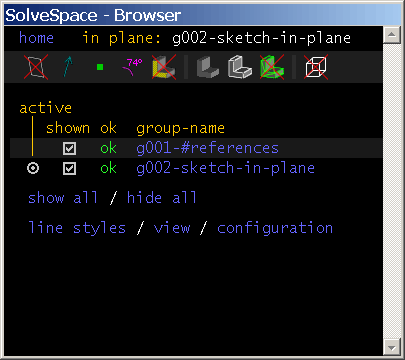
To navigate to a group's page, click that group's name (e.g., "g002-sketch-in-plane"). The links may also trigger actions in the sketch. For example, in the above screenshot, all of the groups are shown. To hide a group, click the box in the "shown" column.

As a convenience, the text window will sometimes automatically navigate to a page that is likely to be relevant. For example, when a new group is created, the text window displays that new group's page. It's always possible to navigate to a different page, by clicking the "home" link at the top left corner (or pressing Esc), and following the links from there.

When sketch entities are selected (e.g., the user has clicked on them with the mouse), information about those entities is displayed in the text window. If a single entity is selected, then information about that entity is displayed. For example, the window display's a circle's center and radius.

If multiple entities are selected, then the text window can sometimes display information about all of them. These cases include:

• two points: the distance between the points
• a point and a plane face: the distance from the point to the plane
• two points, and a vector: the distance between the points, projected along the vector
• two plane faces: the angle between the plane faces

Show / Hide Entities

As the sketch becomes more complex, it may be useful to hide unnecessary information. SolveSpace provides several different ways to do this.

Along the top of the text window, a row of icons appears. These icons make it possible to hide and show different elements in the sketch:

In addition to the above options, it is possible to hide and show entire groups. If a group is hidden, then all of the entities (line segments, circles, arcs, points, etc.) from that group are hidden. The solid model is not affected; if a hidden group contains a circle that is extruded to form a cylinder, then the cylinder will remain visible.

To hide a group, go to the home screen in the text window, by pressing Esc or choosing the link at the top left. A list of groups is displayed, along with their visibility. If a group is visible, then the checkbox in the "shown" column is checked. Click the checkbox; it now appears unchecked, and the group is hidden. The show / hide status of groups is saved in the part file. If a part is linked into an assembly, then entities that were visible in the part file will be visible in the assembly, and entities that were hidden will be hidden.

Active Workplane

SolveSpace represents all geometry in 3d; it's possible to draw line segments anywhere, not just in some plane.

This freedom is not always useful, so SolveSpace also makes it possible to draw in a plane. If a workplane is active, then all entities that are drawn will be forced to lie that plane. The active workplane ("in plane:") is indicated in the top line of the text window, at the right.

When SolveSpace starts with a new empty file, a workplane parallel to the XY plane is active. To deactivate the workplane, and draw in 3d, choose Sketch → Anywhere In 3d.

To activate a workplane, select it, and then choose Sketch → In Workplane. When a workplane is activated, the view is aligned onto that workplane. (The workplane remains active until the user chooses Sketch → Anywhere In 3d, or a different workplane is activated. If the user rotates the view, so that the view is no longer aligned onto the workplane, then the workplane remains active.)

In a "Sketch in New Workplane" group, the group's associated workplane may be activated by choosing Sketch → In Workplane; there is no need to select it first.

Active Group

When a new line, circle, or other curve is created, it will be created in the active group. Geometry from the active group is drawn in white; geometry from earlier groups is drawn in brown. Later groups are hidden.

In the text window's home screen (press Escape, or choose the link in the top left corner), the active group's line in the list of groups has a selected radio button in the "active" column. All other groups (except g001-#references, which cannot be activated) have an unselected radio button in that column. To activate an inactive group, click its radio button.

In order to reduce distraction when sketching in 2D, solid models from inactive groups are "dimmed" (by rendering them using the #def-dim-solid style) so that they blend into the background. To disable this uncheck View → Darken Inactive Solids. By modifying the #def-dim-solid style any color may be assigned to geometry from inactive groups instead of just "dimming" them. A brighter color may even be assigned to this style to make geometry from inactive groups stand out more clearly instead if desired.

Construction Geometry

In normal operation, the user draws line and curves in a sketch. Those curves describe the geometry to be manufactured; ultimately, the endmill or the laser or some other tool will cut along those curves.

In some cases, it is useful to draw a line that should not appear on the final part. For example, the user may wish to draw a center line for a symmetric part; but that center line is only a guide, and should not actually get exported with the CAM data. These lines are called construction lines.

To mark an entity as construction-only, choose Sketch → Toggle Construction. A construction entity will behave just like any other entity, except that it is drawn in green, and does not contribute to the geometry for export by default (or to the section that will be extruded or lathed or swept). You may also toggle construction geometry while sketching a new entity by using the 'g' keyboard shortcut.

Datum Point

This entity is defined by a single point.

If a workplane is active when the datum point is created, then that datum point will always lie in the workplane. If no workplane is active, then the datum point will be free in 3d. (This is the same behaviour as for all points, including e.g. the endpoints of a line segment.)

Datum points are typically used as construction geometry. The user might place datum points in order to simplify the dimensioning of line segments or other entities.

Workplane

This entity is specified by a point and a normal. The point defines its origin, and the normal defines its orientation.

A workplane makes it possible to draw a section in 2d. If a workplane is active, then any entities that are drawn must lie in that workplane.

It's almost never necessary to create workplanes explicitly. Instead, create a new Sketch in New Workplane group.

Line Segment

This entity is specified by its two endpoints. If a workplane is active, then the two endpoints will always lie in that workplane.

To create the line segment, choose Sketch → Line Segment, and then left-click one endpoint of the line. Then release the mouse button; the other endpoint is now being dragged.

To create another line segment, that shares an endpoint with the line segment that was just created, left-click again. This is a fast way to draw closed polygons.

To stop drawing line segments, press Escape, or right- or center-click the mouse. SolveSpace will also stop drawing new line segments if an automatic constraint is inserted. (For example, draw a closed polygon by left-clicking repeatedly, and then hovering over the starting point before left-clicking the last time. The endpoint of the polyline will be constrained to lie on the starting point, and since a constraint was inserted, SolveSpace will stop drawing.)

Rectangle

This entity consists of two vertical line segments, and two horizontal line segments, arranged to form a closed curve. Initially, the rectangle is specified with the mouse by two diagonally opposite corners. The line segments (and points) in the rectangle may be constrained in the same way as ordinary line segments.

It would be possible to draw the same figure by hand, by drawing four line segments and inserting the appropriate constraints. The rectangle command is a faster way to draw the exact same thing.

A workplane must be active when the rectangle is drawn, since the workplane defines the meaning of "horizontal" and "vertical".

Circle

This entity is specified by its center point, by its diameter, and by its normal.

To create the circle, choose Sketch → Circle, and then left-click the center. Then release the mouse button; the diameter of the circle is now being dragged. Left-click again to place the diameter.

If a workplane is active, then the center point must lie in that workplane, and the circle's normal is parallel to the workplane's normal (which means that the circle lies in the plane of the workplane).

If no workplane is active, then the center point is free in space, and the normal may be dragged (or constrained) to determine the circle's orientation.

Arc of a Circle

This entity is specified by its center point, the two endpoints, and its normal.

To create the arc, choose Sketch → Arc of a Circle, and then left-click one of its endpoints. Then release the mouse button; the other endpoint is now being dragged. The center is also being dragged, in such a way as to form an exact semi-circle.

Left-click again to place the other endpoint, and then drag the center to the desired position. The arc is drawn counter-clockwise from the first point to the second.

The arc must be drawn in a workplane; it cannot be drawn in free space.

Tangent Arc at Point

To round off a sharp corner (for example, between two lines), we often wish to create an arc at the corner, that is tangent to both of the lines. This will create a smooth appearance where the line and arc join. It would be possible to draw these arcs by hand, using Sketch → Arc of a Circle and Constrain → Tangent, but it's easier to create them automatically.

To do so, first select a point where two line segments or circles join. Then choose Sketch → Tangent Arc at Point; the arc will be created, and automatically constrained tangent to the two adjoining curves.

The initial line segments will become construction lines, and two new lines will be created, that join up to the arc. The arc's diameter may then be constrained in the usual way, with Distance / Diameter or Equal Length / Radius constraints.

By default, the radius of the tangent arc is chosen automatically. To change that, choose Sketch → Tangent Arc at Point with nothing selected. A screen will appear in the text window, where the radius may be specified. It is also possible to specify whether the original lines and curves should be kept, but changed to construction lines (which may be useful if you want to place constraints on them), or whether they should be deleted.

Bezier Cubic Spline

This entity is specified by at least two on-curve points, and an off-curve control point at each end (so two off-curve points total). If only two on-curve points are present, then this is a Bezier cubic section, and the four points are exactly the Bezier control points.

If more on-curve points are present, then it is a second derivative continuous (C2) interpolating spline, composed of multiple Bezier cubic segments. This is a useful type of curve, because it has a smooth appearance everywhere, even where the sections join.

To create the Bezier cubic spline, choose Sketch → Bezier Cubic Spline. Then left-click one endpoint of the cubic segment. Release the mouse button; the other endpoint of the cubic segment is now being dragged. To add more on-curve points, left click with the mouse. To finish the curve, right-click, or press Esc.

The two control points are intially placed on the straight line between the endpoints; this means that the cubic originally appears as a straight line. Drag the control points to produce the desired curve.

To create a closed curve (technically, a "periodic spline"), start by creating the curve as usual, left-clicking to create additional on-curve points. Then hover the mouse over the first point in the curve, and left-click. The curve will be converted to a periodic spline, which will be C2 continuous everywhere, including at that first point.

Text in a TrueType Font

This entity is defined by four points, at each corner of the text. The distance between the points determines the height and width of the text; the angle of the line between them determines the orientation of the text, and their position determines the text's position.

To create the text, choose Sketch → Text in TrueType Font. Then left-click the top left point of the text. The bottom right point of the text is now being dragged; left-click again to place it.

To change the font, select the text entity. A list of installed fonts appears in the text window; click the font name to select it. To change the displayed text, select the text entity and click the [change] link in the text window.

Image

This entity may be used to place a bitmap reference image in a sketch. The entity is defined by four control points that may be used to position, constrain and orient the image similar to those for TrueType Text entities. Image entities are typically used as a reference for sketching or tracing other entities and removed later. As such, Image entities are not exportable.

Splitting and Trimming Entities

In some cases, it is desirable to draw by creating overlapping figures, and then removing the extra lines. For example, in this case, a circle and a rectangle are drawn; the two short lines and the short arc are then deleted, to form a single closed shape.

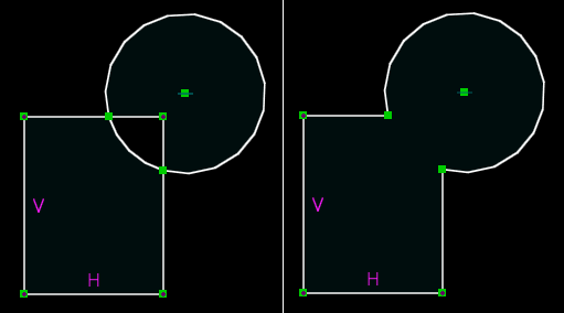
In order to trim the extra lines, it is necessary to split the entities where they intersect. SolveSpace can split lines, circles, arcs, and Bezier curves against each other. To do so, select the two entities to be split, and then choose Sketch → Split Curves at Intersection. This deletes each original entity, and replaces it with two new entities that share an endpoint at the intersection. The excess lines may then be deleted as usual.

Because the original entities are deleted, any constraints on the original entities are deleted as well. This means that the sketch may no longer be constrained as desired after splitting. If an entity is marked as construction before splitting, then it will not be deleted, so the constraints will persist.

General

To create a constraint, first select the geometry to be constrained. For example, when constraining the distance between two points, first select those two points. Then choose the appropriate constraint from the Constrain menu.

Depending on what is selected, the same menu item may generate different constraints. For example, the Distance / Diameter menu item will generate a diameter constraint if a circle is selected, but a length constraint if a line segment is selected. If the selected items do not correspond to an available constraint, then SolveSpace will display an error message, and a list of available constraints.

Most constraints are available in both 3d and projected versions. If a workplane is active, then the constraint applies on the projection of the geometry into that workplane. If no workplane is active, then the constraint applies to the actual geometry in free space.

For example, consider the line shown below:

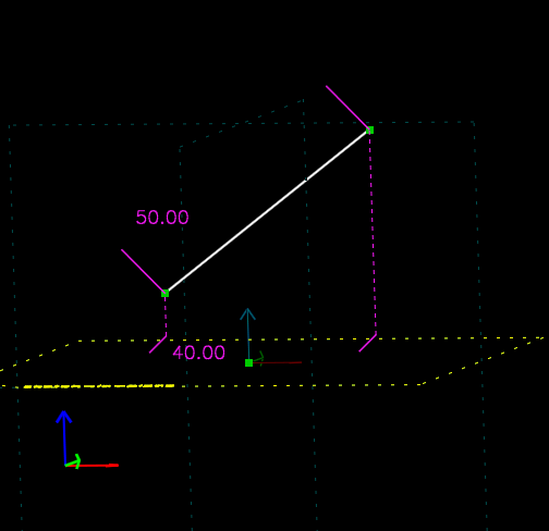
The line's length is constrained in two different ways. The upper constraint, for 50 mm, applies to its actual length. The lower constraint, for 40 mm, applies to the length of its projection into the XY plane. (The XY plane is highlighted in yellow.) The dotted purple lines are drawn to indicate the locations of the line segment's projected endpoints.

In normal operation, the user activates a workplane (or a workplane is activated automatically, for example by creating a "Sketch in New Workplane" group). The user then draws an entity, for example a line. Since a workplane is active, the line is created in that workplane. The user then constrains that line, for example by specifying its length. Since the workplane is still active, the constraint actually applies to the projection of the line segment into the workplane.

In this case, the projected distance is equivalent to the 3d distance. If the line segment lies in the workplane, then the projection of that line segment into the workplane is just that line segment. This means that when drawing in a workplane, most of this can be ignored.

It's possible to use projected constraints in more complex ways, though. For example, the user might create a line segment in workplane A, and constrain its projection into workplane B.

Constraints are drawn in purple on the sketch. If a constraint has a label associated with it (e.g. a distance or an angle), then that label may be repositioned by dragging it with the mouse. To modify the dimension, double-click the label; a text box will appear on the screen, where the new value can be entered. Press enter to commit the change, or Esc to cancel.

Automatic Constraints

There is an option in the configuration screen labled "enable automatic line constraints". If this option is checked and a line being drawn is nearly horizontal, a horizontal contraint will appear over the middle of the line and will be applied when the second point of the line is clicked in place. Similarly when a nearly vertical line is being drawn a "V" constraint will appear automatically. If the line is not close enough to horizontal or vertical, no constraint will be added. Holding Ctrl while sketching will also disable this feature.

If an automatic constraint is redundant or would result in the sketch being over-constrained, it will not be created even if it is shown during line placement. Similarly if a distance or diameter constraint is added that would over-constrain the sketch, it will be created as a reference (REF).

Another option in the configuration screen is "edit newly added dimensions". With this option enabled, when a new Distance, Lenght Ratio, or Length Difference constraint is added the input box will automatically appear so a specific value can be entered. With the option off the user would have to create the constraint and then double-click on it to edit the value, which is almost always what we want to do.

Failure to Solve

In some cases, the solver will fail. This is usually because the specified constraints are inconsistent or redundant. For example, a triangle with internal angles of 30, 50, and 90 degrees is inconsistent--the angles don't sum to 180, so the triangle could never be assembled. This is an error.

A triangle with internal angles constrained to 30, 50, and 100 degrees is also an error. This is not inconsistent, because the angles do sum to 180 degrees; but it's redundant, because only two of those angles need to be specified.

If the sketch is inconsistent or redundant, then the background of the graphics window is drawn in red (instead of the usual black), and an error is displayed in the text window:

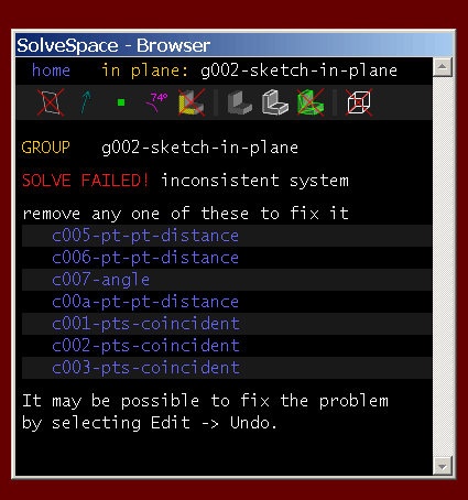
As a convenience, SolveSpace calculates a list of constraints that could be removed to make the sketch consistent again. To see which constraints those are, hover the mouse over the links in the text window; the constraint will appear highlighted in the graphics window. By deleting one or more of the constraints in that list, the user can make the sketch consistent again.

A different type of error occurs when the solver fails to converge. This may be a defect in the solver, or it may occur because impossible geometry was specified (for example, a triangle with side lengths 3, 4, and 10; 3 + 4 = 7 < 10). In that case, a similar error message is displayed, but without a list of constraints to remove to fix things. The problem can be resolved by removing or editing the constraints, or by choosing Edit → Undo.

Reference Dimensions

By default, the dimension drives the geometry. If a line segment is constrained to have a length of 20.00 mm, then the line segment is modified until that length is accurate.

A reference dimension is the reverse: the geometry drives the dimension. If a line segment has a reference dimension on its length, then it's still possible to freely change that length, and the dimension displays whatever that length happens to be. A reference dimension does not constrain the geometry.

To convert a dimension into a reference dimension, choose Constrain → Toggle Reference Dimension. A reference dimension is drawn with "REF" appended to the displayed length or angle. Double-clicking a reference dimension does nothing; the dimension is specified by the geometry, not the user, so it is not meaningful to type in a new value for the reference dimension.

Specific Constraints

To get help on a specific constraint, choose its menu item without first selecting any entities. An error message will be displayed, listing all of the possibilities.

In general, the order in which the entities are selected doesn't matter. For example, if the user is constraining point-line distance, then they might select the point and then the line, or the line and then the point, and the result would be identical. Some exceptions exist, and are noted below.

Distance / Diameter

This constraint sets the diameter of an arc or a circle, or the length of a line segment, or the distance between a point and some other entity.

When constraining the distance between a point and a plane, or a point and a plane face, or a point and a line in a workplane, the distance is signed. The distance may be positive or negative, depending on whether the point is above or below the plane. The distance is always shown positive on the sketch; to flip to the other side, enter a negative value.

Angle

This constraint sets the angle between two vectors. A vector is anything with a direction; in SolveSpace, line segments and normals are both vectors. (So the constraint could apply to two line segments, or to a line segment and a normal, or to two normals.) The angle constraint is available in both projected and 3d versions.

The angle must always lie between 0 and 180 degrees. Larger or smaller angles may be entered, but they will be taken modulo 180 degrees. The sign of the angle is ignored.

When two lines intersect, four angles are formed. These angles form two equal pairs. For example, the pictured lines interesect at 30 degrees and 150 degrees. These two angles (30 and 150) are known as supplementary angles, and they always sum to 180 degrees.

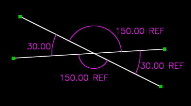
(Notice that in the sketch, three of the angle constraints are reference dimensions. Given any one of the angles, we could calculate the other three; so a sketch that specified more than one of those angles would be overconstrained, and fail to solve.)

When a new angle constraint is created, SolveSpace chooses arbitrarily which supplementary angle to constrain. An arc is drawn on the sketch, to indicate which angle was chosen. As the constraint label is dragged, the arc will follow.

If the wrong supplementary angle is constrained, then select the constraint and choose Constrain → Other Supplementary Angle. A constraint of 30 degrees on one supplementary angle is exactly equivalent to a constraint of 150 degrees on the other.

Horizontal / Vertical

This constraint forces a line segment to be horizontal or vertical. It may also be applied to two points, in which case it applies to the line segment connecting those points.

A workplane must be active, because the meaning of "horizontal" or "vertical" is defined by the workplane.

It's good to use horizontal and vertical constraints whenever possible. These constraints are very simple to solve, and will not lead to convergence problems. Whenever possible, define the workplanes so that lines are horizontal and vertical within those workplanes.

On Point / Curve / Plane

This constraint forces two points to be coincident, or a point to lie on a curve, or a point to lie on a plane.

The point-coincident constraint is available in both 3d and projected versions. The 3d point-coincident constraint restricts three degrees of freedom; the projected version restricts only two. If two points are drawn in a workplane, and then constrained coincident in 3d, then an error will result--they are already coincident in one dimension (the dimension normal to the plane), so the third constraint equation is redundant.

When a point is constrained to lie on a circle (or an arc of a circle), the actual constraint forces the point to lie on the cylindrical surface through that circle. If the point and the circle are already coplanar (e.g., if they are both drawn in the same workplane), then the point will lie on the curve, but otherwise it will not.

Equal Length / Radius / Angle

This constraint forces two lengths, angles, or radiuses to be equal.

The equal-angle constraint requires four vectors as input: the two equal angles are the angle between each pair of inputs. For example, select line segments A, B, C, and D. The constraint forces the angle between lines A and B to be equal to the angle between lines C and D. If the wrong supplementary angle is chosen, then choose Constrain → Other Supplementary Angle, as for the angle constraint.

If a line and an arc of a circle are selected, then the length of the line is forced equal to the length (not the radius) of the arc.

Length Ratio

This constraint sets the ratio between the lengths of two line segments. For example, if line A and line B have length ratio 2:1, then the constraint is satisfied if A is 50 mm long and B is 25 mm long.

The order in which the lines are selected matters; if line A is selected before line B, then the ratio is length of A:length of B.

Length Difference

This constraint sets the difference between the lengths of two line segments. For example, if line A and line B have length difference 5 mm, then the constraint is satisfied if A is 50 mm long and B is 55 mm long or 45mm long.

Note that a negative difference can be entered when editing the constraint to change which is the shorter segment. At the same time the value is always displayed as a positive number (the absolute difference) and entering positive numbers does not change the "direction".

At Midpoint

This constraint forces a point to lie on the midpoint of a line.

The at-midpoint constraint can also force the midpoint of a line to lie on a plane; this is equivalent to creating a datum point, constraining it at the midpoint of the line, and then constraining that midpoint to lie on the plane.

Symmetric

This constraint forces two points to be symmetric about some plane. Conceptually, this means that if we placed a mirror at the symmetry plane, and looked at the reflection of point A, then it would appear to lie on top of point B.

The symmetry plane may be specified explicitly, by selecting a workplane. Or, the symmetry plane may be specified as a line in a workplane; the symmetry plane is then through that line, and normal to the workplane. Or, the symmetry plane may be omitted; in that case, it is inferred to be parallel to either the active workplane's vertical axis or its horizontal axis. The horizontal or vertical axis is chosen, depending which is closer to the configuration in which the points were initially drawn.

Perpendicular

This constraint is exactly equivalent to an angle constraint for ninety degrees.

Parallel / Tangent

This constraint forces two vectors to be parallel.

In 2d (i.e., when a workplane is active), a zero-degree angle constraint is equivalent to a parallel constraint. In 3d, it is not.

Given a unit vector A, and some angle theta, there are in general infinitely many unit vectors that make an angle theta with A. (For example, if we are given the vector (1, 0, 0), then (0, 1, 0), (0, 0, 1), and many other unit vectors all make a ninety-degree angle with A.) But this is not true for theta = 0; in that case, there are only two, A and -A.

This means that while a normal 3d angle constraint will restrict only one degree of freedom, a 3d parallel constraint restricts two degrees of freedom.

This constraint can also force a line to be tangent to a curve, or force two curves (for example, a circle and a cubic) to be tangent to each other. In order to do this, the two curves must already share an endpoint; this would usually be achieved with a point-coincident constraint. The constraint will force them to also be tangent at that point.

Same Orientation

This constraint forces two normals to have the same orientation.

A normal has a direction; it is drawn as an arrow in that direction. The direction of that arrow could be specified by two angles. The normal specifies those two angles, plus one additional angle that corresponds to the twist about that arrow.

(Technically, a normal represents a rotation matrix from one coordinate system to another. It is represented internally as a unit quaternion.)

For example, the picture below shows two workplanes, whose normals are constrained to be parallel:

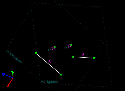
Because the normals are parallel, the planes are parallel. But one plane is twisted with respect to the other, so the planes are not identical. The line on the left is constrained to be horizontal in the leftmost plane, and the line on the right is constrained to be horizontal in the rightmost. These lines are not parallel, even though the normals of the workplanes are parallel.

If we replace the "parallel" constraint with a "same orientation" constraint, then the two workplanes become identical, and the two horizontal lines become parallel.

This is a useful constraint when building an assemblies; a single "same orientation" constraint will fix all three of a linked part's rotational degrees of freedom.

Lock Point Where Dragged

Constrain a point such that the solver will not alter its location. This does not prevent direct manipulation by dragging the entity that owns the point or the point itself. It simply instructs the solver to consider the point fully constrained. This can be easily demonstrated by drawing an equilateral triangle with sides constrained equal and one point locked. Dragging the side opposite this locked point will not alter its position but will resize the triangle instead.

Comment

A comment is a single line of text that appears on the drawing. To create a comment, select Constrain → Comment, and then left-click the center of the new comment. To move the comment, drag it with the mouse. To change the text, double-click it.

The comment has no effect on the geometry; it is only a human-readable note. By default, the comment is shown in the same color as the constraints; but a comment may be assigned to a custom line style, in order to specify the line width and color, text height, text origin (left, right, top, bottom, center), and text rotation.

If a comment is created within a workplane, then the text will be drawn within the plane of that workplane. Otherwise, the text will always be drawn facing forward, in the plane of the screen.

By default, comments are hidden when their group is inactive, the same as for all other constraints. If a comment is assigned to a custom style, then that comment will be shown even when its group is inactive, as long as the style (and the group, and constraints overall) is shown.

To view a list of groups, go to the home page of the text window. This is accessible from the link at the top left of the text window, or by pressing Esc. To view a group's page, click its name in the list.

All groups have a name. When the group is created, a default name (e.g., "g008-extrude") is assigned. The user may change this name; to do so, go to the group's page in the text window, and choose [rename].

Groups that create a solid (e.g. extrudes or lathes) have a "solid model as" option, which is displayed in the page in the text window. The group can be merged as union, which adds material to the model, or as difference, which cuts material away. A third option is intersection, which preserves only the material that falls within both solids.

The union, difference and intersection operations may be performed either as triangle meshes, or as exact NURBS surfaces. Triangle meshes are fast to compute and robust, but they require any smooth curves to be approximated as piecewise linear segments. The NURBS surface operations are not as robust, and will fail for some types of geometry; but they represent smooth curves exactly, which makes it possible for example to export a DXF in which a circular arc appears as an exact circle, instead of many piecewise linear edges.

These groups also have a color, which determines the color of the surfaces they produce. To change the color, click one of the swatches in the group's page in the text window.

The group's page in the text window also includes a list of all requests, and of all constraints. To identify a constraint or a request, hover the mouse over its name; it will appear highlighted in the graphics window. To select it, click the link in the text window. This is equivalent to hovering over and clicking the actual object in the graphics window.

Sketch in 3d

This creates a new empty group, in which the user may draw lines, circles, arcs, and other curves.

The ultimate goal is usually to draw closed sections (like a triangle, or a square with a circular cutout, or some more complicated shape). These sections are the input for later groups. For example, an extrude group takes a flat section, and uses it to form a solid.

If all of the entities in the group can be assembled into closed loops, then the area that the loops enclose is shaded in very dark blue. This is the area that would be swept or extruded or lathed by a subsequent group.

Sketch in New Workplane

This creates a new empty group, similar to a new "Sketch in 3d". The difference is that a "Sketch in New Workplane" also creates a workplane. The workplane is created based on the entities that are selected when the sketch is created. These may be:

The new group's associated workplane is automatically set to be the active workplane.

If the entities in this group do not form closed curves, then an error message is displayed on the screen, and a red line is drawn across the gap. An error is also displayed if the curves are not all coplanar.

Step Translating

This group takes geometry in the active group, and copies it multiple times along a straight line.

If a workplane is active when the step translating group is created, then the translation vector must lie parallel to that workplane. Otherwise, the translation vector may go anywhere in free space.

The number of copies to create is specified by the user. To change this value, click the [change] link in the group's page in the text window.

The copies may be translated on one side, or on two sides. If the copies are translated on one side, then the original will appear to the left of (or above, below, etc.) all the copies. If the copies are translated on two sides, then the original will appear in the center of the copies.

The copies may be translated starting from the original, or starting from copy #1. If the translation starts from the original, then the translation will contain the original. (So a 1-element step will always produce the input geometry in its original location.) If the translation starts from copy #1, then the original is not included in the output. (So a 1-element step makes a single copy of the input geometry, and allows the user to translate it anywhere in space.)

If the active group is a sketch (sketch in 3d, sketch in new workplane), the the sketch is stepped and repeated. In that case the user would typically draw a section, step and repeat that section, and then extrude the step and repeat.

If the active group is a solid (extrude, helix, lathe, revolve), then the solid is stepped and repeated. In this case, the user would draw a section, extrude the section, and then step and repeat the extrusion.

In some cases, these two possibilities (extrude the step, vs. step the extrusion) are equivalent. If the translation vector isn't parallel to the section plane, then only the second option will work.

Step Rotating

This group takes the geometry in the active group, and copies it mutiple times along a circle.

Before creating the group, the user must select its axis of rotation. One way to do this is to select a point, plus either a line segment or a normal; the axis of rotation goes through the point, and is parallel to the line segment or normal.

If a workplane is active, then it's also possible to select just a point; in that case, the axis of rotation goes through that point, and is normal to the workplane. This means that the rotation remains within the plane of the workplane.

The step and repeat options (one side / two sides, with original / with copy #1) are the same as for step translating groups.

The numer of copies is specified in the same way as for step translating. If the rotated geometry has not yet been constrained, then the copies will be spaced evenly around a circle; for example, if 5 copies are requested, then the spacing will be 360/5 = 72 degrees.

To place the copies along less than (or more than) a complete circle, drag a point on one of the copies with the mouse; all of the rest will follow, as the step rotation angle is modified. Constraints (for example an angle constraint, or a point-on-lie constraint) may be used to specify the angle of rotation exactly.

Extrude

This group takes a flat section, and extrudes it to form a solid. The flat section is taken from the section of the group that is active when the extrude group is created. (This is usually a sketch in workplane, or a sketch in 3d, but could also be a step and repeat.)

The sketch may be extruded on one side, or on two sides. If the sketch is extruded on one side, then the new solid is either entirely above or entirely below the original sketch. Drag a point on the new surface to determine the extrude direction, and also to determine the extrude depth. Once the extrusion depth looks approximately correct, it may be specified exactly by using constraints. For example, the user might constrain the length of one of the newly extruded edges.

If the sketch is extruded on two sides, then the original sketch lies at the exact midpoint of the new solid. This means that the solid is symmetric about the original sketch plane. Later dimensioning often becomes simpler when the part has symmetry, so it's useful to extrude on two sides whenever possible.

A workplane must be active when the group is created, and the extrude path is automatically constrained to be normal to that workplane. This means, for example, that a rectangle is extruded to form a rectangular prism. The extrusion has one degree of freedom, so a single distance constraint will fully constrain it. It is possible to extrude perpendicular to a workplane other than the one the sketch is drawn in by selecting the other workplane prior to creating the extrusion. This can be used to create skewed extrusions.

By default, no workplane is active in a new extrude group. This means that constraints will apply in 3d; for example, a length constraint is a constraint on the actual length, and not on the length projected into some plane. This is typically the desired behaviour, but it's possible to activate a workplane in the usual way (by selecting it, then choosing Sketch → In Workplane).

Lathe

This group takes a flat sketch, and sweeps it around a specified axis, to form a solid of revolution. The section is taken from the group that is active when the lathe group is created.

To create a lathe group, first select a line segment. Then choose New Group → Lathe. The line segment is the axis of revolution.

The section must not intersect itself as it is swept along the curve. If the section crosses the axis of rotation, then it is certain to intersect itself and fail.

Revolve

This group takes a flat sketch, and sweeps it around a specified axis, to form a solid of revolution. The difference between this and a Lathe group is that Revolve does not sweep a full 360 degrees. The resulting solid can be dragged or constrained to a specific angle. If dragged beyond 360 degrees this will produce the exact same solid as a Lathe group.

Helix

This group takes a flat sketch, and sweeps it around a specified axis while also translating along that axis. The result is a helical surface which can be used to model threads or other twisted surfaces. The two most common approaches are to use an axis in the sketch plane to create a spiral shape, or an axis perpendicular to the sketch plane to create what behaves like a twisted version of the standard extrusion.

When a Helix group is created, a construction line will also be created along the axis of the helix. Dragging the ends of that line or any other points on the axis will change the length of the helical extrusion. Dragging points that are not on the axis will change the angle of the helix similar to a Revolve group. The angle of a helix can be much more than 360 degrees to allow creation of very long spiral shapes, or all of the threads on a bolt in a single group.

Link / Assemble

In SolveSpace, there is no distinction between "part" files and "assembly" files; it's always possible to link one file into another. An "assembly" is just a part file that links one or more other parts.

The linked file is not editable within the assembly. It is included exactly as it appears in the source file, but with an arbitrary position and orientation. This means that the linked part has six degrees of freedom.

To move (translate) the part, click any point on it and drag it. To rotate the part, click any point and Shift+ or Ctrl+drag it. The position and orientation of the part may be fixed with constraints, in the same way that any other geometry is constrained.

The part may also be transformed with a 3Dconnexion six degree of freedom controller. To manipulate a part in an assembly, select any entity within that part (for example, a point, a line segment, or a normal). The 3Dconnexion controller will move that part, instead of transforming the view. Be careful not to produce an undesired translation into or out of the screen, since that motion may not be readily perceptible.

To rotate the part by exactly ninety degrees about the coordinate axis (x, y, or z axis) closest to perpendicular to the screen, choose Edit → Rotate Imported 90°. If an entity in a linked group is selected, then the part from that group will be rotated. If an import group is active, then the part from the active group will be rotated.

The Same Orientation constraint is particularly useful when linking parts. This one constraint completely determines the linked part's rotation. (Select a normal on the linked part, select some other normal to constrain it against, and choose Constrain → Same Orientation).

The linked part also has an associated scale factor. This makes it possible to link a smaller or larger version of the part. If the scale factor is negative, then the part is scaled by the absolute value of the scale factor and mirrored.

SolveSpace also has the ability to import IDF (.emn) files defining printed circuit boards from electronic design tools. This is useful for designing enclosures and checking fit within an assembly. Sketch entities and an extrusion of the board will be created and can be used for taking measurements.

Import groups have a special "solid model as" option: in addition to the usual "union", "difference" and "intersection", they have "assemble". The "assemble" option should be used when combining parts that should not interfere with each other into an assembly. To verify that the assembly does not interfere, choose Analyze → Show Interfering Parts.

If an import group contains a sketch that forms a closed contour, then that group may be extruded in the same way as if the contour had been drawn within the same file. This means that it is possible to draw a section in file A, import that section into file B (with some arbitrary translation and rotation), and then extrude it to form a feature of the part in file B. Any changes to file A will propagate into file B when the part is regenerated.

Similarly, it's possible to draw an open section in file A, link that section into file B, and then draw additional lines or curves (in the same group or another group) within file B to close that section. If file C links in file B, then the closed section may be extruded. This allows the user to reuse sections, or portions of a section, in multiple files, in such a way that a change in the original will propagate to all the parts that use that geometry.

When an assembly file is loaded, SolveSpace loads all of the linked files as well. If the linked files are not available, then an error occurs. When transfering an assembly file to another computer, it's necessary to transfer all of the linked files as well.

It is never possible to change a line or curve's color, line width, or other cosmetic properties directly. Instead, the cosmetic properties of an entity may be specified by assigning that entity to a line style. The style specifies color, line width, text height, text origin, text rotation, and certain other properties that determine how (and whether) an object appears on-screen and in an exported file.

SolveSpace's basic color scheme is defined by the default styles. To view them, choose "line styles" from the home screen in the text window. This is where, for example, lines are specified to be white by default, and constraints to be magenta, and points to be green. The default styles may be modified. These modifications will be saved in the user config (the registry on Windows, a .json file on other platforms), and will apply to all files opened on that computer.

It is also possible to create custom styles, for cosmetic or other purposes. (For example, laser cutters often use the color of a line to specify the power and feed with which to cut it.) To create a custom style, choose "new custom style" in the style screen. The new style will appear at the bottom of the list of styles, with default name new-custom-style.

To modify a style, click its link in the list of styles. Color is specified as red, green, blue, where each component is between 0 and 1. The line width may be specified either in pixels, or in inches or millimeters. If the line width is specified in pixels, then the line width in an exported file will depend on the on-screen zoom level. If the user zooms out (so that the model appears smaller on screen), then the geometry shrinks but the lines, measured in pixels, stay the same size; this means that lines will appear thicker compared to the model in the exported file.

Entities (like lines, circles, or arcs) may be assigned to a line style. One way to do so is to enter the desired line style's screen in the text window, and then select the desired entities. Then click the "assign to style" link in the text window. Another way to do so is to right-click the entity, and assign it to the style using the context menu.

Comments (Constrain → Comment) may also be assigned to styles. The style may be used to specify the text height, the rotation of the text in degrees, and from what point (top, bottom, left, right, center) the text is aligned. The snap grid (View → Show Snap Grid, Edit → Snap to Grid) is often useful when creating cosmetic text.

User-created styles are saved in the .slvs file, along with the geometry. If a part with user-created styles is linked in, then the styles are not imported; but the style identifiers for the linked in entities are maintained. This means that the user can specify the line styles in the file doing the linking (i.e., the "assembly").

If a style is hidden, then all objects within that style will be hidden, even if their group is shown. If a style is not marked exportable, then objects within that style will appear on-screen, but will not appear in an exported file. This behavior is similar to that of construction lines.

Not all export file formats support all line style information. For example, lines in an HPGL file are exported without any line width or color.

Trace Point

SolveSpace can draw a "trail" behind a point as it moves. This is useful when designing mechanisms. The sketch shown below is a four-bar linkage:

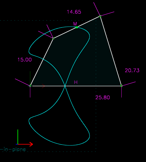
As the linkage is worked, the midpoint of the top link moves along the cyan curve. This image was produced by drawing the linkage, tracing that midpoint, and then dragging the linkage through its full range of motion with the mouse.

To start tracing, select a point, and choose Analyze → Trace Point. When the point moves, a cyan trail will be drawn behind it.

To stop tracing, choose Analyze → Stop Tracing. A dialog will appear, with the option to save the trace as a CSV (comma-separated value) file. To save the trace, enter a filename. To abandon the trace, choose Cancel or hit Esc.

The trace is saved as a text file, with one point per line. Each point appears in the format x, y, z, separated by commas. Many programs, including spreadsheets like Excel, can read this format. The units for the coordinates are determined by the export scale factor. (If the export scale factor is 1, then they are millimeters, and if it's 25.4, then they're inches.)

If the mechanism is worked by dragging it with the mouse, then the points in the trace will be unevenly spaced, because the motion of the mouse is irregular. A plot of x vs. y (like the cyan trace above) is not affected, but a plot of x or y vs. t is useless, because the "speed" along the curve is not constant.

To avoid this problem, move the point by stepping a dimension, rather than by dragging with the mouse. Select the dimension to be stepped; this can be any distance or angle. Choose Analyze → Step Dimension. Enter the new final value for that dimension, and the number of steps; then click "step dimension now".

The dimension will be modified in multiple steps, and solved at each intermediate value. For example, consider a dimension that is now set to 10 degrees. The user steps this dimension to 30 degrees, in 10 steps. This means that SolveSpace will solve at 12 degrees, then 14 degrees, then 16, and so on, until it reaches 30 degrees.

The position of the traced point will be recorded at each intermediate value. When the trace is exported, it represents the position of that point, as the dimensioned link rotates with constant angular speed.

The step dimension feature can also improve convergence. In some difficult cases, the solver will fail to find a solution when a dimension is changed. If the specified constraints have multiple solutions, then the solver may also find an undesired solution. In this case, it may be useful to try stepping the dimension to its new value, instead of changing it in a single step.

Measure Volume

This feature reports the volume of the part. Depending on the active units, the volume is given in cubic inches, or in millilitres and cubic millimeters.

If the part contains smooth curves (e.g. circles), then the mesh is not an exact representation of the geometry. This means that the measured volume is only an approximation; for a mesh that looks fairly smooth on-screen, expect an error around one percent. To decrease this error, choose a finer chord tolerance.

Measure Area

This feature reports the area of the current sketch. Depending on the active units, the area is given in square inches, or in square millimeters.

The area measurement is calculated using a piecewise linear approximation to any curves. This introduces some error; to decrease that error, choose a finer chord tolerance. If the current sketch is not a well-formed plane curve (for example, if it isn't a closed curve, or if it intersects itself) then an error is reported, because the area cannot be defined.

Show Degrees of Freedom

This feature indicates which points in the sketch are not completely constrained (i.e., which points would move if the user dragged them with the mouse). The free points are drawn with a large cyan square over them. In a sketch with zero degrees of freedom, nothing would be drawn. In a sketch with one degree of freedom, one or more points would be marked; it's possible that more than one point would be marked, since that one degree of freedom might be draggable via multiple points.

To erase the large cyan squares, re-solve the sketch by choosing Edit → Regenerate All or by dragging a point.

Bitmap Image

This option will export a bitmap image of whatever is displayed on-screen. It is equivalent to taking a screenshot. This option is useful for producing human-readable output.

Choose File → Export Image. The file is exported as a PNG, which most graphics software can open.

2d Section

This option will cut the solid model along a specified plane. All lines and curves from the solid model that lie in this plane will be exported. Lines and curves from the solid model that do not lie in this plane are ignored. Lines and curves that do not come from the solid model (for example, a line in a sketch that has not been extruded) are ignored. This option is typically appropriate when generating 2d CAM data from a 3d model, for example for a laser or waterjet cutter.

Before exporting a section, it is necessary to specify which plane of the part should be exported. This may be specified by:

The units of the exported file are determined by the export scale factor, which may be specified in the configuration screen.

If the sketch contains curves, then the exported file may represent those curves exactly (for example, a circle in an SVG file, since SVG supports exact circles), approximately but with a smooth curve (for example, a circle in a PDF file, since PDF supports only cubic splines, which can't represent a circle exactly), or as piecewise linear segments (for example, a circle in an HPGL file). To force curves to be output as piecewise linear, choose "curves as piecewise linear" in the configuration screen. Colors in the output file may not exactly match colors of the model viewed on-screen, depending on the color space used by your viewer.

2d View

This option will project the 3d model onto a plane, in the same way that it is projected when you view the model on screen. Lines and curves that happen to lie in the projection plane are exported without any changes; lines and curves that do not lie in the projection plane will appear shortened due to the projection.

This option is typically appropriate when generating a human-readable drawing in vector format. It is also useful because it exports all lines, not just lines from the solid model; so if the user draws a sketch from lines and curves, but does not wish to extrude it to form a solid model, then they can extrude their bare sketch using this option. This may be desirable when using SolveSpace for 2d drawing.

The projection plane is selected by rotating the model on-screen, by center-dragging with the mouse. The origin of the exported file corresponds to the center of the view on screen, and may therefore be moved by panning (by right-dragging with the mouse). To specify the projection plane exactly, orient the view onto a workplane, or use the View → Nearest Ortho / Iso View and View → Center View at Point commands.

By default, the view will be output with hidden lines removed, and additional lines will be drawn wherever a curved surface turns from front-facing to back-facing. This is typically the desired result. To create a wireframe view of the part, show "hidden-lns" before exporting.

Some file formats (EPS, SVG, PDF) support shaded surfaces. If the user is exporting to such a file format, and the "export shaded 2d triangles" option is set in the configuration screen, then the view will contain flat-shaded surfaces of the model. Lighting is calculated in the same way as for the view of the model on-screen. It may therefore be modified by changing the light directions and intensities in the configuration screen.

The units of the exported file are determined by the export scale factor, which may be specified in the configuration screen. If hidden line removal is performed (for example, if a solid model is present), then the exported file will contain only line segments; all curves are broken down into lines, with the specified chord tolerance. If no hidden line removal is performed (for example, if nothing has been extruded or lathed, so no solid model is present) then curves will be exported in exact form when possible.

Normals, datum points and image entities are not exported for vector formats.

3d Wireframe

This option behaves almost identically to File → Export 2d View; but instead of projecting the lines and curves into the specified 2d plane, it exports the lines and curves in 3d.

The 3d wireframe does not contain any surfaces or solids. This means that it is generally not appropriate for the viewing or manufacturing of solid parts. For that, use a triangle mesh or a NURBS surface (STEP) file.

Triangle Mesh (STL, OBJ)

This option will generate a 3d triangle mesh that represents the entire part. Most 3d CAM software, including the software for most 3d printers, will accept an STL file.

The mesh from the active group will be exported; this is the same mesh that is displayed on screen. The coordinate system for the STL file is the same coordinate system in which the part is drawn. To use a different coordinate system (e.g., to rotate or translate the part), create an assembly with the part in the desired position, and then export an STL file of the assembly.

The units of the STL file are determined by the export scale factor, which may be specified in the configuration screen.

NURBS Surfaces (STEP)

If the model is represented as NURBS surfaces (and not just as a triangle mesh), then the user can export those exact surfaces as a STEP file. When this is possible, it is usually the best choice, since it does not introduce any error. Many CAM, rapid prototyping, and other CAD tools will accept a STEP file.

The STEP file will always indicate millimeter units, no matter what scale factor is applied.

Material Colors

In the text window screen for certain groups (extrude, lathe, sweep), a palette of eight colors is displayed. This palette allows the user to choose the color of any surfaces generated by that group.

These eight colors are specified here, by their components. The components go from 0 to 1.0. The color "0, 0, 0" is black, and "1, 1, 1" is white. The components are specified in the order "red, green, blue".

A change to the palette colors does not change the color of any existing surfaces in the sketch, even if the color of an existing surface no longer appears in the palette.

Light Directions

The 3d part is displayed with simulated lighting, to produce the impression of depth. There are two types of lights, directional and ambient. The directions and intensities of these lights may be modified according to user preference.

Directional lights do not have a position; they have only a direction, as if they were coming from very far away. This direction is specified in 3 components, "right, top, front". The light with direction "1, 0, 0" is coming from the right of the screen. The light with direction "-1, 0, 0" is coming from the left of the screen. The light with direction "0, 0, 1" is coming from in front of the screen. The ambient light has no direction and acts as a fill light of uniform intensity from all directions.

The intensity must lie between 0 and 1. A light with intensity 0 has no effect, and 1 is full brightness. Lighting from ambient and directional lights is additive. If the ambient light intensity is set to 1 a "flat shading" effect will be achieved.

Two directional lights are available. If only one is desired, then the second may be disabled by setting its intensity to zero. When the part is rotated or translated, the lights do not move.

Chord Tolerance, and Max Segments

SolveSpace does not always represent curved edges or surfaces exactly. Curves are sometimes broken down into piecewise linear segments, and surfaces are sometimes broken down into triangles.

This introduces some error. The chord tolerance determines how much error is introduced; it is the maximum distance between the exact curve and the line segments that approximate it. If the chord tolerance is decreased, then more line segments will be generated, to produce a better approximation.

There are two chord tolerance values in the configuration screen. The first is specified as a percent of the overall size of the sketch and its value in length units is also calculated and shown. This means a sketch consisting of a single circle will have very smooth curves, while a large object with small holes may have fewer segments because the hole is much smaller than the overall sketch and closer in size to the chord tolerance.

The second value is the "export chord tolerance" which is an absolute value in mm. When exporting a triangle mesh for 3d printing or g-code for machining, this value will determine how much the resulting part can deviate from the ideal curved surfaces.

When combining NURBS surface or triangle meshes from different groups, SovleSpace uses the chord tolerance in some calculations. That means when a boolean operation fails, making adjustments to the chord tolerance can "fix" the problem in some cases.

The fineness of the mesh is also limited by the specified maximum number of piecewise linear segments. A single curve will never be broken down into more than that number of line segments, no matter how fine the chord tolerance.

Perspective Factor

To display a 3d part on-screen, it must be projected into 2d. One common choice is a parallel projection. In a parallel projection, any two lines that are parallel in real life are also parallel in the drawing. A parallel projection is also known as an axonometric projection. Isometric and orthographic views are examples of parallel projections.

Another way to transform the image into 2d is with a perspective projection. In a perspective projection, objects closer to the "camera" appear larger than objects that are farther away. This means that some lines that are parallel in real life will not be parallel in the drawing; they will converge at a vanishing point.

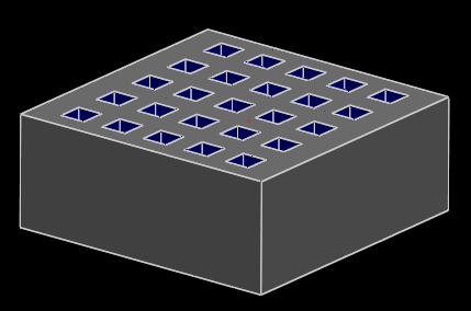
The image below is a perspective projection. All of the square cutouts are the same size, but the ones at the front (closer to the viewer) are drawn larger, and the ones at the back are drawn smaller.

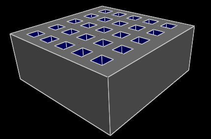
The next image is a parallel projection. All of the square cutouts are the same size on the drawing. (The cutouts at the top might look slightly larger, but that is an optical illusion, because the eye is accustomed to seeing images with perspective.)

A perspective projection will often look more realistic, and gives a better impression of depth. The disadvantage is that the perspective distorts the image, and may cause confusion.

By default, SolveSpace displays a parallel projection. To display a perspective projection, choose View → Use Perspective Projection, and make sure that the perspective factor is not zero. By default, the perspective factor is 0.3. The distance from the "camera" to the model is equal to one thousand pixels divided by the perspective factor.

Snap Grid Spacing

This specifies the pitch of the snap grid, in inches or millimeters. By default, the grid is not displayed; it may be shown by choosing View → Show Snap Grid. Points are never automatically snapped to the grid. To snap a point, select that point, and then choose Edit → Snap to Grid. Comments (Constrain → Comment, cosmetic text) may be snapped to grid in the same way.

Export Scale Factor

Internally, SolveSpace represents lengths in millimeters. Before exporting geometry, these lengths are divided by the export scale factor. This scale factor determines the units for the exported file.

If the scale factor is set equal to 1, then exported files are in millimeter units. If the scale factor is set equal to 25.4, then the exported files are in inch units, since 1 inch = 25.4 mm.

SolveSpace works in a right-handed coordinate system. If the scale factor is negative, then the exported file will appear in a left-handed coordinate system (so that a right-handed screw thread will become left-handed, and text would appear mirrored).

Cutter Radius Offset

When exporting a 2d view or section, this option may be used to apply cutter radius compensation. All curves in the exported geometry are offset by the specified radius. This may in some cases make it possible to work without dedicated CAM software.

The cutter radius is specified in inches or millimeters, according to the current mode. To disable cutter radius compensation, set this offset to zero.

The cutter radius compensation works only on piecewise linear segments. This means that curves (circles, Beziers, etc.) will be approximated as line segments in the output file, even if "curves as piecewise linear" is set to "no".

Export Shaded 2d Triangles

When exporting a view of the part, the user can export only the edges of the part (to produce a wireframe or hidden line removed drawing), or the user can export flat-shaded surfaces, to show the color and lighting of the faces of the part.

Not all export file formats support shaded triangles; currently, SVG, EPS, and PDF do, but DXF and HPGL do not.

Export Curves as Piecewise Linear

A smooth curve (like a circle, or a Bezier curve) may be exported in one of two ways: either exactly, or as a set of line segments that approximates it. If this box is not checked, then whenever possible, geometry will be output as exact curves. If it is checked, then curves will always be exported as piecewise linear segments.

This option is useful because some CAM or other software is incapable of importing exact curves, but almost all software will be capable of importing piecewise linear segments.

Export Canvas Size

This specifies the canvas size for any exported 2d geometry. For example, the canvas size in a PDF file is the paper size, and the canvas size in a PostScript file is the EPS BoundingBox. This may be specified in one of two ways: either as a fixed size, or as a set of margins around the exported geometry.

Fix White Exported Lines

By default, SolveSpace draws white lines on a black background. But most export file formats assume a white background, which means that white lines would be illegible. By default, SolveSpace will rewrite any white (lighter than approximately 75% gray) colors to black when exporting into such a file format. That behavior may be disabled with this option.

Draw Triangle Back Faces in Red

SolveSpace always works with solid shells. This means that in normal operation, only the outside of a surface should be visible. This setting should therefore have no effect.

If a self-intersecting shell is drawn, then inside surfaces may be exposed. Even if the shell is watertight, a few stray pixels from an inside surface may "show through", depending on how the graphics card renders triangles. This setting determines whether those surfaces are discarded, or drawn highlighted in red.

Check for Closed Contours

Most solid operations (like extrudes and lathes) work only on closed, planar sections that are not self-intersecting. By default, SolveSpace will warn the user if the sketched section violates any of these rules, by indicating the problem on the sketch. For example, if a contour is open, then a message is drawn at one of the hanging endpoints. If a contour is self-intersecting, then a message is drawn at the intersection.

For general 2d and 3d wireframe CAD work, this behavior may not be desired. The warnings may therefore be disabled with this option.

G Code Parameters

SolveSpace is not a CAM program, but it is capable of exporting simple G code for 2d parts. By applying the correct cutter radius compensation (or by drawing the sketch with the cutter radius in mind), it is possible to profile 2d parts with no additional CAM software. The part is assumed to lie in the XY plane. The cutting depth along the Z axis is as specified here; enter a positive or negative value, depending on which sign corresponds to down. The top of the workpiece is assumed to lie at Z = 0, and the cutter will move to a clearance plane 5mm above the workpiece while slewing.

All units are in either inches or millimeters (or inches or millimeters per minute, for the feeds), according to the current mode.

When Boolean operations are performed on triangle meshes (instead of exact NURBS surfaces), the resulting mesh quality will often be poor. An equally good mesh might have been achieved with fewer triangles, if the curves were piecewise-linear approximated differently. Or the mesh may contain long skinny triangles.

This means that the exported STL files will not contain a high quality mesh. This is generally not a problem, but could be in some applications. In particular, the exported mesh may no longer be exactly 2-manifold (i.e., watertight). Check for this problem with Analyze → Show Naked Edges.

Another consequence is that the program runs slower as the number of triangles increases. It's a good idea to draw with a fairly coarse mesh. Before exporting, reduce the chord tolerance; the part will be regenerated with a finer mesh.

When Boolean operations are performed on NURBS surfaces, the mesh quality will in general be much better. But some types of surface intersection are not handled by the current NURBS Booleans, so it may in some cases be impossible to perform the desired operation as a NURBS Boolean.

The NURBS Booleans are also affected by the chord tolerance. Operations may fail if that tolerance is too coarse, but the routines become slower as the tolerance gets finer. If problems occur, then it is often useful to change that tolerance.

To improve speed and mesh quality, draw the part using fewer Boolean operations. For example, a plate with a hole might be modeled in two different ways. The user might extrude the plate, and then cut a hole by extruding a circle as difference. Or the user might draw a single sketch with both the outline of the plate and the hole, and extrude only once. The latter option is preferable. The trim command (Sketch → Split Curves at Intersection) may be useful while drawing complicated sections.