
In this tutorial, we will take multiple parts, and combine them into a parametric assembly. We will place the parts within the assembly using constraints. Once we've defined the assembly, we can verify that no parts interfere with each other, and generate multiple 2d or 3d representations of that assembly. With a careful choice of constraints, we will define the assembly in such a way as to permit us to modify the original parts, and have those changes propagate correctly into our assembly.
Any SolveSpace file can be linked into any other SolveSpace file; there is no special type for parts or assemblies. This means that sub-assemblies, for example, work in the obvious way. We could draw any of our parts from scratch, but they are also available for download pre-drawn:
Extract these files to a directory somewhere on your computer. It's possible to link files from any directory into any file, but for simplicity it is best to put the parts and assembly in a single directory. If we do this, then we can copy that single directory to another computer and retain all the parametric links between the files.
We can open any of these files to view them. All of these are simple 2d parts, that could be laser-cut or three-axis milled from 6mm or 3/8" acrylic. They are designed to assemble with tabs in slots, to form a box with six compartments:
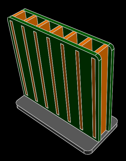
We wish to assemble these parts—a base, two sides, and seven dividers—into that box. To do so, we will begin with the base. (Of course, we could begin with any component that we wanted. But it's logical to begin with the base.) Create a new file in SolveSpace by choosing File → New. In that new file, choose New Group → Link / Assemble. Specify the base.slvs file that you just saved on your computer. (You may also use New Group → Link Recent, if base.slvs appears in that list. This is exactly equivalent.)
The part will appear in our assembly. We can grab any point with the mouse, and left-drag; the entire part will move along with us, within the plane of the screen. We can rotate our view of the part (in the usual way, by center-dragging with the mouse) to see where we've dragged the part in 3d. So by left-dragging points on the model, we can translate the part within the assembly.
We also can grab a point with the mouse, and Shift+left-drag. This rotates the part into and out of the plane of the screen, about that point. We can similarly rotate the part by left-dragging any of the blue arrows that represent normals. And to rotate the part within the plane of the screen, we can Ctrl+left-drag either a point or a normal.
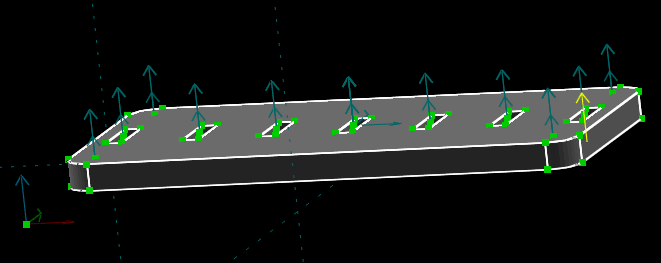
It's difficult to precisely define the orientation or position of a part within an assembly using the mouse. So it's best to just place the part roughly, and then define its exact position using constraints. To start, place the base in roughly the position shown above, close to the coordinate axes. The X, Y, and Z axes are drawn as dark red, green, and blue arrows here respectively. (The coordinate axes also appear at the bottom left of the graphics window at all times, drawn in bright red, green, and blue. They behave identically no matter which copy is used.)
To start, we would like to define the orientation of the part. We can do that by locking one of the part's normals in the same orientation as one of our coordinate axes. Here, a good choice would be to constrain any of the base's normals—which are drawn as blue arrows—in the same orientation as our coordinate system's Z axis, which is also drawn as a blue arrow, in this view pointing approximately up from the origin. Select those two normals by left-clicking them, and choose Constrain → Same Orientation, or the equivalent constraint from the toolbar.
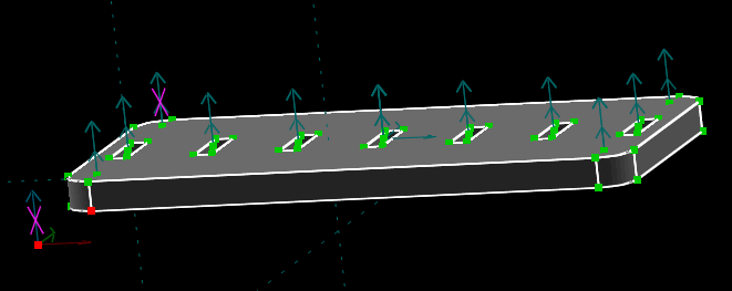
The two normals are now each marked with a magenta X, which is visible above. (It doesn't matter which of the normals on the part were chosen to constrain, since they all point in the same direction. The choice is arbitrary.) This means that those two normals are constrained to point in the same direction (i.e., parallel); but it also locks the twist of the part about that axis, so it fully constrains the part's orientation. The same-orientation constraint is useful, because it completely specifies a part's orientation with a single constraint.
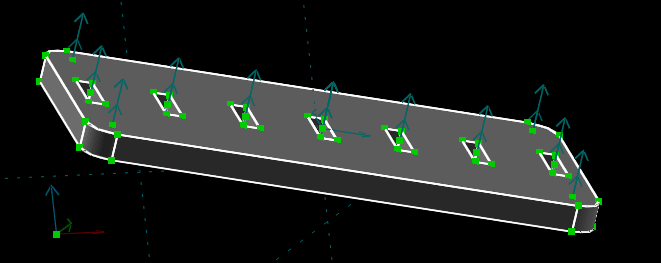
We can try to drag the part's orientation and rotation now. We will find that it is still possible to translate the part anywhere, but impossible to rotate it, because that rotation is now fixed. To define the translation, we can use a point-coincident constraint. Select the two points marked in red in the image above, and choose Constrain → On Point. The two points will now be constrained to be coincident, locking the linked part's translation. The imported part is now fully constrained.
Next, we wish to place the seven dividers. We will again choose New Group → Link / Assemble, and specify divider.slvs. The divider will appear in our assembly, initially with the wrong position and orientation. We therefore must drag it into roughly the position indicated below, with the longer of the divider's two tabs aligned to the slot on the base. We can do this with the mouse, by left-dragging the position and Shift+left-dragging the orientation. It may also be useful to choose Edit → Rotate Imported 90°, to rotate the linked part by exactly ninety degrees about the coordinate axis that's closest to normal to the screen. (So if we are looking onto the XY plane, for example, then it rotates the part about the Z axis.)
As before, we can lock the orientation of the divider with a same-orientation constraint on one of its normals. One possible choice is to lock a normal on the divider against our coordinate system's X axis, which is drawn in red. The magenta X marks are again visible on the image below, indicating the two normals that are in the same orientation.

And we have again indicated two points in red that could be constrained coincident to define the position of the part. Select those two points by left-clicking them, and choose Constrain → On Point. The divider is now fully constrained.
We could repeat this process six more times, to place the seven dividers. But it's easier to step and repeat our one linked part seven times. So choose New Group → Step and Repeat Translating. By default, three copies of the original part will appear, stepped along some constant distance and direction:

Note that we have now hidden points and normals, by clicking the respective icons at the top of the Property Browser. The assembly is getting more complex, so those were cluttering the screen. We can show or hide those as desired at any time.
In the step and repeat group's Property Browser screen (press Tab to show that window if it is hidden), we can change the number of times repeated to seven. We now see seven copies of that divider. We can drag these copies with the mouse. The first one is locked, and the orientation of all of them is locked (since the first copy's orientation is locked, and the copies have a different translation but the same rotation). But by dragging any of the other copies, we can change the translation distance and direction for the step and repeat.

We can drag the parts into roughly the correct position, and then, as usual, place the exact position using a constraint. Above, select the two points that are shown marked in red. (Even when points are hidden, they will appear when the mouse is hovered over them, and may be selected by left-clicking in the usual way.) Constrain those two points coincident, and the seven dividers will be placed as desired.

Finally, we wish to place the two sides. We choose New Group → Link / Assemble as usual, and specify side.slvs. It appears within our assembly with some arbitrary position and orientation, which are probably not what's desired.

In this particular default position and orientation, it is interfering with other parts in the assembly. This is obvious, though we could choose Analyze → Show Interfering Parts to confirm that. Press Esc to clear the red error lines.
Drag and rotate the side into roughly the position indicated below; once again, Edit → Rotate Imported 90° may be a better way to define the orientation than by Shift+left-dragging with the mouse.

Once again, constrain the orientation of the linked part using a same-orientation constraint, for example on one of that part's normals against our coordinate system's Y axis (drawn in green). Note that it does not matter if the Y axis and part's normal are pointing in exactly opposite directions; the constraint will constrain them either parallel or anti-parallel, depending on which is closer to the initial configuration.
We could again use a point-coincident constraint to define the orientation of the part, and that would in fact be the simplest way to do so. But to illustrate different types of constraint, we will instead use three point-on-face constraints.
The plane faces of the parts are selectable; they are highlighted with a yellow stipple pattern when the mouse hovers over them, and appear with a red stipple pattern when they are selected. Here, we have selected a face on the inside of one of the slots on the green side, and a point on the orange divider. If it is difficult to select the faces because other entities are getting highlighted instead, then try zooming in more.

Select Constrain → On Plane; the part may now move only in such a way as to maintain that point within the plane of that face. Rotate the view into several different orientations (by middle-dragging with the mouse) and try dragging the part. As drawn here, it will be possible to move the part in the Y and Z directions, but not the X direction. So if the view is roughly aligned to the YZ plane, for example, then the part will seem to have two degrees of freedom, but if the view is aligned to the XY plane then it will seem to have only one. Of course, the part actually has two degrees of freedom; it started with three translational degrees of freedom, and the point-on-face constraint has subtracted one.

Next, select the plane of the top of the grey base and a point on the bottom of the green side, as indicated in the image above. Again choose Constrain → On Plane. The part now has only one degree of freedom, and may be dragged only parallel to the Y axis. Finally, select the outer face of the green side, and a point on the outside of one of the orange divider's tabs, as indicated below.

Again constrain the point on the face. The green side's position is now locked. Point-on-face constraints are useful when constraining assemblies, because each constraint subtracts only a single degree of freedom. This is useful when constraining an assembly only partially, for example if we wish to drag the parts and produce an exploded view. It's often difficult to drag a part's three degrees of freedom if its position is left completely unconstrained, but if the part is constrained with only a single degree of freedom, then it's possible to drag that one degree of freedom with less confusion.
Parts may be placed with any constraint in SolveSpace, not just point-coincident or point-on-face constraints. Those two constraints are typically the most useful, though. A point-on-line constraint, for example, subtracts two degrees of freedom. This means that two point-on-line constraints are an error, since they must overconstrain the part (which has only three translational degrees of freedom, when the two constraints are trying to subtract four degrees of freedom). The combination of a point-on-line constraint and a point-on-face would be correct (2+1 DOF), or a point-on-line constraint plus a point-on-line constraint projected into a workplane (since the projected version of the constraint removes only one degree of freedom), or many others.
It's possible to constrain the position and orientation of parts in SolveSpace in many different ways. In general, though, it should almost always be possible to constrain the parts with same-orientation, point-coincident, and point-on-face constraints only.
Note in particular that it's not possible to place the position and orientation (six degrees of freedom) of a part using two point-coincident constraints. It seems like this should work, because the part initially has six degrees of freedom, and each point-coincident constraint removes three degrees of freedom. But the part, with those constraints, would obviously still be free to rotate about the line connecting the two constrained points. So that combination of constraints fails to fully constrain the part's rotation, and overconstrains the part elsewhere. It is therefore invalid.
Place the other side of the box by any method; for example by linking it again and using a same-orientation and point-coincident constraint, or by stepping and repeating the side that we've just place twice, or in some other way.

The assembly is now complete. We can view it on-screen, and produce isometric (View → Nearest Isometric View) or top, bottom and side (View → Nearest Ortho View) views of all the parts. We can suppress the display of a part by changing that setting in its Property Browser screen. For example, to hide the base, we would click the home link at the top of the Property Browser, and then choose its group—which in our assembly was the first import group, g003-import—from the list of groups. We then click the box labeled "suppress this group's solid model" to check it. To show that part again, we click that box again to uncheck it.
We can verify that no parts interfere by choosing Analyze → Show Interfering Parts. If any parts interfere, then red lines will be drawn to indicate the location of the interference. (Note that this operation works on the triangle mesh, and not the exact NURBS surfaces; this means that it is guaranteed to work only for plane surfaces, and might report an erroneous interference for a round pin in a round hole.)
Note that Analyze → Show Naked Edges will show many errors. This is expected, and not a problem. In our assembly, we have many places where two parts lie against each other exactly. The parts are supposed to fit together exactly, so this is the desired behavior; but a mesh that has two triangles exactly coplanar with each other is an error, so the "STL check" properly fails. For assemblies, Show Naked Edges is not typically meaningful; use Show Interfering Parts instead.
We can export views of the assembly in the same way that we would export a view of a part. For example, we can choose File → Export View to produce a hidden-line-removed PDF, as shown below.

(We had been working with parallel projections of the model so far, but this drawing has some perspective. We added this by choosing View → Use Perspective Projection. To adjust the amount of perspective, change the perspective factor in the configuration screen. The configuration screen is reachable from the link at the bottom of the home screen in the Property Browser.)
We can make changes to one of the parts, and then regenerate the assembly (by choosing Edit → Regenerate All, or by closing and reopening the file). The changes will propagate into our assembly, and with a careful choice of constraints, the parts will remain assembled in the desired configuration.
This completes our tutorial. The assembly is also available for download:
Note that if you download the assembly, then it is necessary to extract all the part files to the same directory as the assembly file before attempting to open the assembly file. The assembly file does not contain a copy of the parts, so the program must rescan the part files every time it regenerates.
To learn more about SolveSpace, including the assembly features, see the other tutorials or the reference manual.